A Guide Through Generative Models - Index

Dear fellow machine learner, this series of articles will explore some Unsupervised Learning algorithms with a focus on generative systems capable of reproducing new data not existing in the original dataset.

• Part 1 : Bayesian Inference and Single Mode Learning - This article
• Part 2 : Improving Bayesian Inference with Multi-Modes learning - Coming Soon
• Part 3 : Variational AutoEncoders: Deep Learning with Bayes - Coming Soon
• Part 4 : Generative Adversarial Neural Networks aka. GANs - Coming Soon

1. Rapid Overview of Unsupervised Learning and Generative AI

1.1 Supervised vs Unsupervised Learning

Most of the classical and widely-known techniques in Machine Learning fit in the realm of Supervised Learning. They usually pursue one of these two goals: classification (i.e. predicting a label/category) or regression (i.e. predicting a numerical value). The key idea in Supervised Learning is that a model is trained to map some entries (i.e. data) with some specific output(s).

In contrast, Unsupervised Learning does not focus on learning to map an input with an output. It is an objective which mostly tries to discover or learn the data distribution. Therefore, Unsupervised Learning is mostly used to perform clustering or data generation.

1.2 Generative Models and sampling from a latent space

As stated before, Unsupervised Learning is strategy which focuses on learning a data-distribution, the distribution of the input data. Once this step is achieved, the learnt distribution can be used to generate new samples that come from the same (or a similar-looking) data distribution.

1.2.1 How can a distribution allow me to generate new data points ?

Let us consider this simple example:
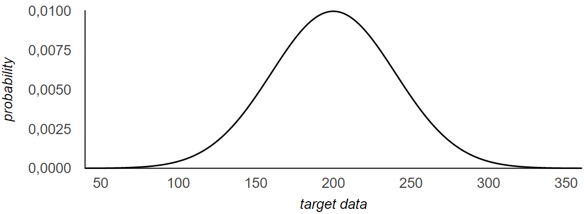
A gaussian distribution defined as followed: \(x \sim \mathcal{N} (200, 40)\). The chart below will allow you to visualise its probability density function also called pdf. This chart represents the probability that any point that comes from this distribution has a specific value.

To Be Noted: A Gaussian Distribution is also called a Normal distribution.

Knowing this distribution, is there any way to generate a data point that follows the given distribution ?

Absolutely! And this is a very simple process:

1. Uniformly and randomly sample from \(z\) the latent space, \(z \in [0, 1]\).
2. Use the percent point function (also called ppf) of the normal distribution which gives the following mapping: \(f: z \mapsto x\)

Alright, let's try this in python now:

import scipy.stats
import numpy as np

def generate_new_data(mu, sigma):
    z = np.random.rand() # Uniformly randomly chosen value in [0, 1]
    return z, scipy.stats.norm(mu, sigma).ppf(z) # ppf : Percent Point Function

# ================= Sanity Checks =================
my_distribution = scipy.stats.norm(200, 40)

test1 = np.round(my_distribution.ppf(0.5))
test2 = np.round(my_distribution.ppf(0.5 + 0.3413))
test3 = np.round(my_distribution.ppf(0.5 + 0.3413 + 0.1359))

print("Test 1 (should give: 200) = %d" % test1)
# >>> Test 1 (should give: 200) = 200
print("Test 2 (should give: 200 + sigma = 240) = %d" % test2)
# >>> Test 2 (should give: 200 + sigma = 240) = 240
print("Test 3 (should give: 200 + 2 * sigma = 280) = %d" % test3)
# >>> Test 3 (should give: 200 + 2 * sigma = 280) = 280

# ======== Let's sample 5 new data point ==========
for _ in range(5):
    print("Latent Variable: z = %.3f => Result: x_new = %.2f" % generate_new_data(200, 40))

# >>> Latent Variable: z = 0.268 => Result: x_new = 175.35
# >>> Latent Variable: z = 0.779 => Result: x_new = 230.87
# >>> Latent Variable: z = 0.757 => Result: x_new = 227.93
# >>> Latent Variable: z = 0.776 => Result: x_new = 230.39
# >>> Latent Variable: z = 0.346 => Result: x_new = 184.14

All of this can be done a bit more rapidly using only numpy (even if it is a bit less comprehensive):

import numpy as np

for _ in range(5):
    print("Result: x_new = %.2f" % np.random.normal(200, 40))

# >>> Result: x_new = 238.21
# >>> Result: x_new = 199.43
# >>> Result: x_new = 206.17
# >>> Result: x_new = 153.71
# >>> Result: x_new = 242.44

In summary, we have sampled uniformly \(z\) from the latent space, with \(z \in [0, 1]\). Then we use the ppf function to transform the randomly chosen sample into actual target data similar to the dataset used to learn the distribution.

Congratulation! You just have generate your first data sample from a learned distribution.

2. Using Bayes Classifier as a Generative Model

The Bayes Classifier is maybe one of the most widely known Machine Learning model. However, it is more frequently used as a classifier, and today this is not our focus.

Alright, so can I use the Bayes Classifier to generate new data ?

For the following we will use the following notations:

• \(x\): the input data.
• \(y\): the data label.
• \(p(x|y)\): probability of x given its label y (i.e. knowing that the label of \(x\) is \(y\))
• \(p(x|y=1)\): probability of x given its label \(y=1\) (i.e. knowing that the label of \(x\) is \(y = 1\).)
• \(p(y|x)\): probability of y given a data point x => classification objective!

In the list above, you will recognise \(p(y|x)\) that one will focus to perform classification. However this article focus on generative models, thus, we will focus on learning \(p(x|y)\). In short, our objective will be to learn for each class \(y_i\) the following conditional probability: \(p(x|y == y_i)\).

2.1. Overview of the complete process from a theoretical perspective

2.1.1. Training the Bayes Classifier to learn the data distribution

Disclaimer: In order to simplify the problem, we will consider, in this article, that all the data we have follow a gaussian distribution. It would be wise to actually check this assumption or at least try other credible distributions in real situations.

In order to learn the data distribution, our objective will be to fit a Gaussian to the data for each label and thus to learn the distribution \(p(x|y == y_i)\) as a Gaussian for each label noted \(y_i\).

In order to learn \(p(x|y == y_i)\), we will process as followed for each label \(y_i\):

1. Find all the data points \(x_i\) that belong to the class \(y_i\).
2. Compute the following:
   1. \(\mu_{y_i}\) = mean of those \(x_i\).
   2. \(\sigma^2_{y_i}\) = covariance of those \(x_i\).

2.1.2. Choosing a label at random to generate with the learned distribution \(p(x|y)\) a new data point.

In order to sample a new data point, we firstly need to choose from which label (i.e. \(y_i\)) we want it to be generated.

Problem: What if the dataset is unbalanced (i.e. \(y_a\) is more frequent than \(y_b\))?

Example: we have \(40%\) of data with the label 'A' and $60% with label 'B'? It seems obvious that we randomly pick a label, it will give us a biaised situation generating more data with label 'A' than it should have to.

Solution: Instead of randomly sampling from a uniform distribution, we can learn the distribution of \(y\) and sample from it:

2.1.3. Now that you know how to choose a label \(y\), let's implement this!

First, you need to download the dataset: MNIST.

As I want to keep it as easy as possible, let's use the version hosted on Kaggle:

1. Download the file train.csv on the Kaggle website (an account required): https://www.kaggle.com/c/digit-recognizer/data
2. Extract the file and place it in your project folder in the folder "data" => myProject/data/train.csv

Second, we will need the following libraries, make sure you have them installed.

• numpy => Numerical and Mathematical Operation
• pandas => Manipulating Data and Tables => DataFrames
• matplotlib => Displaying Data, Visualisation and Images

Let's go for Python and Bayes !

Disclaimer: This tutorial has been designed and tested for Python 3 only.

We need to import all the libraries we will need...

import os
from builtins import range, input

import numpy as np
import pandas as pd
from numpy.random import multivariate_normal as mvn

import matplotlib.pyplot as plt

Next step, we will define a function to load the data for us:

def get_mnist():
    if not os.path.exists('data'):
        raise Exception("You must create a folder called 'data' in your working directory.")

    if not os.path.exists('data/train.csv'):
        error = "Looks like you haven't downloaded the data or it's not in the right spot."
        error += " Please get train.csv from https://www.kaggle.com/c/digit-recognizer"
        error += " and place it in the 'data' folder."
        raise Exception(error)

    print("Reading in and transforming data...")

    # We use the pandas library to load the training data.
    df = pd.read_csv('data/train.csv')
    data = df.as_matrix()

    # We shuffle our dataset in order to be sure that the data comes in a random order
    np.random.shuffle(data)

    # We create two variables X and Y containing the data (X) and the labels (Y)
    X = data[:, 1:] / 255.0 # pixels values are in [0, 255] => Normalize the data
    Y = data[:, 0]          # the first column contains the labels

    print("Data Loading process is finished ...")

    return X, Y

Next step, we will define a class: BayesClassifier. This class will expose a few methods:

1. fit(): fit the model to the data
2. sample_given_y(): sample from the given \(y\) class.
3. sample(): sample from any \(y_i\) randomly chosen (according to the distribution of y).

class BayesClassifier:
    def fit(self, X, Y):
        # assume classes ∈ {0, ..., K-1}
        self.K = len(set(Y))

        self.gaussians = list()

        for k in range(self.K):
            Xk   = X[Y == k]         # We get all the Xi of class k
            mean = Xk.mean(axis=0)   # We compute their mean
            cov  = np.cov(Xk.T)      # We compute their covariance

            self.gaussians.append({
                "m": mean,
                "c": cov
            })

    def sample_given_y(self, y):
        g = self.gaussians[y]
        return mvn(mean=g["m"], cov=g["c"], tol=1e-12)

    def sample(self):
        y = np.random.randint(self.K)
        return self.sample_given_y(y)

Last step, we will load the data and train the model. Expect it to last around 2-3 minutes.

We will actually learn the mean and covariance of each class \(y_i\). As we have 10 different digits, we will repeat this process 10 times. At each time we will display the mean image and a random sample from this \(y_i\).

X, Y = get_mnist()
clf = BayesClassifier()
clf.fit(X, Y)

for k in range(clf.K):
    # show one sample for each class and the mean image learned in the process

    sample = clf.sample_given_y(k).reshape(28, 28) # MNIST images are 28px * 28px
    mean   = clf.gaussians[k]["m"].reshape(28, 28)

    plt.subplot(1, 2, 1)
    plt.imshow(sample, cmap="gray", interpolation="none") # interpolation is added to prevent smoothing
    plt.title("Sample")

    plt.subplot(1, 2, 2)
    plt.imshow(mean, cmap="gray", interpolation="none")
    plt.title("Mean")

    plt.show()

Results:

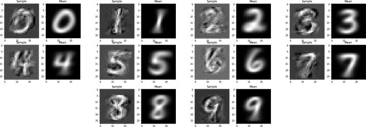
It is quite logical that the mean image is completely blurry because this image is average of all the images of class \(y_i\). It seems that the model did quite well his job, let us investigate how good is the data generation.

# generate a random sample
samples = list()

col_number = 4
row_number = 10

img_size   = 2.0

fig_size = plt.rcParams["figure.figsize"] # Current size: [6.0, 4.0]

fig_size[0] = img_size * col_number # width
fig_size[1] = img_size * row_number # heigh

fig, axes = plt.subplots(row_number, col_number)
fig.subplots_adjust(hspace=0.1)

for _ in range(col_number*row_number):
    row = _ // col_number
    col = (_ - row*col_number)
    axes[row, col].imshow(clf.sample().reshape(28, 28), cmap="gray", interpolation="none")
    axes[row, col].axis('off')

plt.rcParams["figure.figsize"] = fig_size

Results:

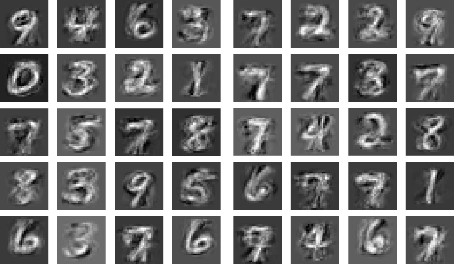
Congratulation! You did it! You finally trained your first generative model.

There is no systematic way to judge on a scale generated data, however I think we can definetely think that the examples generated looks defintely like handwritten digits even if it doesn't really look like genuine data.

In my opinion, we can say that the results are quite incredible for just an incredibly simple model. To be honest, I wouldn't have thought that BayesClassifier could give that (good) kind of results for a generative task.

D. Conclusion

We have seen in this article how to generate new data samples, however they do not look very good. We will explore in the upcoming articles how to improve these results and obtain more realistic generated sampled. One of the solution could be multi-mode learning with Gaussian Mixture Models, explored in Part 2 - Stay Tuned!

• Part 1 : Bayesian Inference and Single Mode Learning - This article
• Part 2 : Improving Bayesian Inference with Multi-Modes learning - Coming Soon
• Part 3 : Variational AutoEncoders: Deep Learning with Bayes - Coming Soon
• Part 4 : Generative Adversarial Neural Networks aka. GANs - Coming Soon

Acknoledgment

I would like to thank two friends for proof-reading and correcting my article: Gaetan Blondet and Emeric Ostermeyer.
It was really helpful and I am really thankful for the time you both have taken. I owe you some drinks!